Alloys, Microstructures and Phase Diagrams

With some of the basics of material crystal structure out of the way, we can move on to a more detailed discussion of alloys and microstructures. Here, I'll focus on the binary iron-carbon system, the most basic components of all steel alloys and cast iron. The solid solution formed is probably the most widely studied system in materials science and one of the most common engineering materials out there. It also makes for an interesting comparison to the common body of knowledge that trades like blacksmithing developed long before the formal background work was done.

The Equilibrium Phase Diagram

Let’s start with a binary phase diagram, a diagram that shows the various phases a binary (two-component) material system can form. Specifically, we’ll look at the \(\mathrm{Fe-Fe}_3\mathrm{C}\) or iron-cementite phase diagram: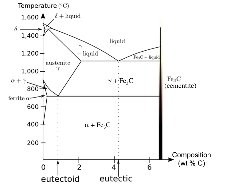

Iron-carbon equilibrium phase diagram, with approximate temperature-color guide.

 This is the portion of the larger phase diagram for the iron-carbon system most relevant to steels. Now let’s look at some of its details.

Moving from left to right the fraction of carbon increases, from zero (pure iron) to a maximum of about 6.7 wt% (percent by weight) carbon. In practice this composition range is where all steels and cast irons lie. Typically the line between steel and cast iron is drawn at about 2.1 wt% C, with the cast irons falling above 2.1 wt% C. So-called ‘mild steels’ are low carbon content steels found at 0.05-0.3 wt% C. ‘high-carbon’ steels are typically considered to be those with 0.3-1.7 wt% C.  The right-most phase, \(\mathrm{Fe_3C}\), is also known as cementite.

The solid lines in the phase diagram indicate phase boundaries, in other words: thermodynamic equilibrium between the phases present on either side of the boundary (this is essentially Gibbs Phase Rule in graphic form). Within the solid lines, the label indicates the phases present. For example, at the left-most side we see solid solutions of the different phases of iron (\(\alpha\) or ferrite, \(\delta\), and \(\gamma\) or austenite) with carbon as the solute. We also see the liquid phase (L) at the top of the diagram. The line that separates the liquid phase from the mixed liquid/solid phases (such as \(\gamma + L\)) is called the liquidus, while the line that separates the mixed liquid/solid phases from the solid-only phases is called the solidus. The region between these two sets of lines reflects the fact that the melting point of a solid solution varies with composition, and that you can have equilibrium between a liquid phase and a solid phase of the same material.

In the iron-carbon system, there is a point at about 4.3 wt% carbon and 1147 °C, where the liqidus meets the solidus. In other words, upon cooling (or 'quenching') from above the melting point the liquid solidifies into two solid phases. This point is called the eutectic point, and the composition at which this point occurs is called the eutectic composition. If a sample of material at this composition was cooled slowly, the resulting microstructure would be alternating layers of the two solid phases. In the iron-carbon system, this would look like the following:
\[ \mathrm{L_{4.3wt\% C}} \rightarrow \gamma\mathrm{-Fe} + \mathrm{Fe_3C}\]
The resulting two-phase microstructure is called ledeburite, and is well into the cast iron category based on carbon content.

Another important point occurs when a single solid phase is cooled and transforms into two different solid phases. The point at which this type of transition occurs is called a eutectoid (as in 'like the eutectic') point. In the iron-carbon phase diagram, there is a eutectoid at about 0.76 wt% carbon and a temperature of about 727 °C. The transformation on slow cooling from just above this temperature would look like:
\[\gamma\mathrm{-Fe} + \mathrm{0.76wt\% C} \rightarrow \alpha\mathrm{-Fe} + \mathrm{Fe_3C}\]
the resulting microstructure of alternating regions of ferrite and \(\mathrm{Fe_3C}\) is called pearlite. The presence of cementite increases the strength and hardness over the ferrite alone, but at the cost of ductility and toughness. However, the phase is able to be drawn into fine, and very strong, wires that are used in a number of applications, including suspension bridges.

Pearlite in a ferrite matrix, courtesy of wikimedia commons.

Non-Equilibrium Phases

In the pearlite transformation, the slow cooling allows the microstructure to do what it needs to do to reach its most energetically favorable (i.e. stable) state, or very close to it. So What would happen if we were to cool the material very rapidly?

The short, and not very useful, answer is: it depends on exactly what you did. Two major things can occur: phase changes at temperatures not predicted by the equilibrium phase diagram boundaries, and the creation of non-equilibrium phases that do not show up on the equilibrium phase diagram. Let's dig into some examples:

Bainite (and a bit more on Pearlite)

Let's start with a sample of an iron-carbon solid solution at the eutectoid composition (0.76 wt% C), at a temperature just above the eutectoid point (727 °C). If we were to cool this sample extremely rapidly (say in 0.5 second) to a temperature between 215 °C and 540 °C, and hold it at that same temperature for a period of time (depending on the temperature, from 10 s to about 14 hours), we'd form a microstructure consisting of small parallel strips or needles of ferrite in a matrix of \(\mathrm{Fe_3C}\). This structure, which is distinct from pearlite though the constituents are the same, is called bainite.

Bainite in a weld zone of a mild steel. Image courtesy of Wikimedia Commons

We can visualize this process, as well as the competitive process of pearlite formation from austenite on a diagram called an isothermal transformation diagram or time-temperature-transformation (T-T-T) diagram:

Isothermal transformation diagram for a iron-carbon alloy of eutectoid composition. The letters  indicate specific phases: austenite (A), pearlite (P), bainite (B), and martensite (M). The solid blue lines indicate two cooling paths resulting in 100% pearlite (top) and 100% bainite (bottom). Modified from image from aarontan.org

In the above diagram, we find 4 different phases: austenite (A), pearlite (P), bainite (B), and martensite (M). The black dotted line at about 540 °C is the separating temperature line between the pearlite and bainite phases. The left-most 'C' curve (red in the image) is the start of the austenite to pearlite or bainite transformation, while the right-most curve (green in the image) is the completion of the transformation. In between, the dotted line indicates 50% completion. Note that the distance between the two 'C' curves changes with temperature, indicating a change in the amount of time required for the transformation to complete. At temperatures above about 700 °C, the pearlite transformation does not complete, meaning there is always some austenite remaining.

On the diagram there are two blue lines: the upper illustrates an isothermal transformation to pearlite, while the lower illustrates a transformation to bainite. The first portion of each curve indicates the rapid cooling to the transformation temperature, while the second is the isothermal hold or soak lasting on the order of several minutes. If the soak length was changed such that the soak ended between the C-curves, the fraction of the transformed phase could be determined from the soak time relative to the time required for completion (but remember: the time axis is logarithmic). For example, below is a diagram showing the creation of a 25% bainite, 75% austenite structure:

Isothermal transformation of an austenitic sample at the eutectic point to 25% bainite. Accomplished through rapid cooling to 450 °C, then holding for about 8 seconds and rapidly cooling to room temperature. Modified from image from aarontan.org

And here's a slightly complicated cooling scheme, that results in 50% pearlite and 50% bainite. Note how the second heat treatment step resets the time by jogging back along the time axis. This is sort of a short hand to indicate the reference time has reset, since the time axis really is soak time at the given temperature.

Diagram showing a two-stage isothermal heat treatment that results in 50% pearlite and 50% bainite. Modified from image from aarontan.org

In the above diagram, the two-stage isothermal heat treatment is performed as follows: First, the 100% austenite sample is quickly cooled to 650 °C and held until 50% of the original austenite has transformed into pearlite. Then, the sample is rapidly cooled to about 440 °C (with little transformation occurring) and held until all of the remaining austenite (50% of the original amount) is transformed into bainite. Then the sample is rapidly cooled to room temperature preventing further transformation.

From a mechanical properties perspective, the ferrite needles tend to have a great number of mobile dislocations present. This results in a gradual yielding behavior in bainite, similar to that seen in pearlite.

Spheroidite

Let's begin with a pearlitic or bainitic microstructure, and heat it to around 700 °C, and maintain it at that temperature for about 30 hours and quickly cool it to room temperature. The long duration spent at such an elevated temperature allows the carbon to diffuse readily, producing a structure consisting of nearly spheroidal particles of \(\mathrm{Fe_3C}\) in a continuous matrix of either pearlite or bainite based on the starting sample. This structure is called spheroidite, the most ductile microstructure of steel.  It also possesses a high fracture toughness because the hard \(\mathrm{Fe_3C}\) particles tend to stop or slow crack propagation, but has a lower hardness than pearlite.

Martensite

The third major microstructure for iron-carbon alloys, known as martensite, is formed during rapid cooling of austenitic microstructure to low temperatures. The rate of cooling must be sufficiently high that there is little time for diffusion to occur. Instead, coordinated motion of iron atoms results in a distortion of the BCC structure of austenite to a body-centered-tetragonal structure. Therefore the formation of martensite is called a 'diffusion less transformation'.

(Schematic of the BCC to BCT transformation that occurs when martensite is formed from austenite. The BCT structure is just a BCC structure that has been elongated along one lattice vector. The carbon atoms would sit in one of the interstitial sites.

The microstructure of martensite in iron-carbon alloys comes in two main forms: lath (or massive) and lenticular (or plate). Lath martensite consists of blocks of parallel blades of the martensite phase separated by the untransformed austenite (or other phases). This type of martensite is common for alloys containing less than about 0.6 wt% C. For higher carbon alloys,  lenticular martensite forms, where the martensite takes on a lens or lenticular shape within the untransformed matrix.

Image of lenticular martensite, optical micrograph after acid etching. White is the untransformed austenite. Image courtesy of wikimedia commons.

Unlike the previous microstructures, maintaining a sample at a specific temperature after the formation process has begun does not form additional martensite. Because the transformation is nearly instantaneous, the fraction of martensite created depends only on the temperature to which the material is cooled. So while it does appear on the isothermal transformation diagrams as we saw earlier, it is much more convenient and realistic to discuss it in terms of a constant cooling rate, which is represented in continuous cooling transformation (CCT) diagrams.

Continuous cooling transformation diagram for a iron-carbon alloy of eutectoid composition. Note that this is not quite the same diagram as the isothermal diagram for the same composition. Modified from image from aarontan.org.

What we can see in the diagram are two important cooling rates (assuming a constant cooling rate): one fast rate that is the minimum required cooling rate for the sample to entirely transform to martensite (called the 'critical cooling rate'), and a slower rate in which no martensite is formed and instead you have only pearlite. For rates between these, you'll have a mixture of pearlite and martensite. We don't see a bainite portion on this plot because it shifts to longer times compared to the isothermal transformation diagram, resulting in all of the available austenite transforming to pearlite before the bainite transformation is possible. For other compositions, this changes such that in some alloys a bainite transformation is possible.

From a material properties perspective, martensite is the hardest, strongest and most brittle form of steel. Because of this, it is often created in carefully controlled quantities in a mixed microstructure (usually with pearlite or austenite) so as to balance the improved strength and hardness with the decrease in ductility.

Effect of Other Alloying Elements

Steel is generally never simple iron and carbon, often containing small quantities of metals such as chromium (Cr), vanadium (V), manganese (Mn), nickel (Ni), molybdenum (Mn), and a variety of other elements. There are a number of reasons that other alloying elements are used; chief among them is to move certain portions of the phase or transformation diagrams, so that specific microstructures can be created.  Other reasons include corrosion resistance, improved heat-treatability and modified mechanical properties (generally via microstructural changes).

Naming Conventions

If you've ever spent much time looking at a catalog of steel alloys, it becomes obvious really quickly that there's a whole bunch of them. Because of this, there are specific naming conventions used for steel alloys, most commonly (in the US at least) the American Iron and Steel Institute (AISI)/Society for Automotive Engineers (SAE) steel grade system. This system uses a 4 number designation where the first digit indicates the primary alloying element (other than carbon), the second indicates the secondary alloying element and the last two digits are the weigh percentage of carbon (in hundredths of a percent). For example: 1060 steel is a plain high carbon steel with 0.60 wt% C. Common mild steels are the 1006 through 1026 (all plain carbon steels). Spring steels include the medium carbon content steels such as 1074, 1075, as well as higher carbon content 1095 and others: the main distinguishing feature of these steels is the ability to obtain a high yield strength, increasing the elastic deformation capabilities. It is important to note that the 4-digit designation itself does not indicate processing, though specific alloys may often be processed in certain ways when purchased in certain forms.

Though we didn't talk about aluminum in this post, there is a similar naming scheme for aluminum alloys that you've probably seen before. The most common designation is that specified by the Aluminum Association, which uses a 4 digit number for wrought alloys, along with a designation for specific heat treatments. For example: 6061-T6 is an aluminum alloy with magnesium and silicon as the major alloying elements that has been solution heat treated and artificially aged. As an aside, 6061 alloys are only called 'aircraft aluminum' because they are actually used for some plane bits and it sounds cool on the box of a flashlight or bike. I could just as meaningfully call them 'bicycle aluminum' or 'flashlight aluminum', but those don't sell as many planes.

For historical interest, here's a photo of some of the documentation that ALCOA used to produce for their product line. My father was able to get me a set of them at one point when the design department was dumping them:

Books like these are already relics in the engineering world, as most things  like this are now done with electronic resources. These ones are circa 1967, and are definitely not the oldest technical texts in my shelf. The leather conditioner was just me being lazy when taking the picture.

How Do You Actually Get a Phase Diagram or Transformation Diagram?

In the above discussion, I only talked about plain carbon alloys at the eutectoid composition. This is mainly for convenience, though that is also a useful and interesting point from a materials science perspective. The closest alloys are probably AISI 1074 and 1075, high-carbon, low alloy (plain) steels whose allowed carbon content fall right near the ideal 0.76 wt% C. But how about all those other alloys?

Well, the simple answer is you contact the manufacturer to find out if they have the diagrams available, or look it up on the internet. Most common alloys will likely be easy to find, though they may be behind paywalls.

But how are those determined?

Fine question. The answer is they are determined through a combination of experimental and theoretical work. One method that is widely used in materials science to obtain phase diagrams for complicated systems is the CALPHAD approach. The quick and dirty of this approach is this: it uses a database mining method to develop 'simple' functions for the Gibbs free energy of various phases, based on tabulated coefficients for a specific functional form. From the model for the free energy based on these coefficients, it performs a minimization to determine where the phase boundaries and produces the graphical phase diagram.

Transformation diagrams, on the other hand, require knowledge of the changes in the system under specific conditions, and are generally determined from a large number of experiments.

Some Historical Context

One of the things I find amazing is that for systems as complex as steels and bronze alloys, metal artisans around the world were able to skillfully obtain items with the desired properties, literally millenia before the formal work I describe above was laid out. The concept of free energy as discussed by Willard Gibbs wasn't around until the 1870s, while the discovery of steel can be dated back to 1400 BC, with iron and bronze work being even older. Yet we have many extant pieces indicating a rather detailed understanding of what is required to get a particular property.

It would be a mistake to take something like a note to use fresh young yak's blood or doe urine to quench a blade, or to sing a particular tune while heating a piece as being a quaint bit of mysticism. In the case of the quenching fluids, the thermal properties and chemical compositions may be surprisingly consistent between urine of young does in a specific area: it's those that matter, but it wasn't like the blacksmith in medieval France could just order himself up a custom quenching fluid from Ye Olde Dow Chemical. For the singing: what easier and more portable way is there to track time when the stopwatch hasn't even been invented? I've already covered why using color was actually a fantastic way to estimate temperature before anyone invented a thermometer that could withstand the abuse.

I admit that this is one area in which I am woefully undereducated: my engineering education really never got much into the history of the field itself beyond a few notes about particular individuals or processes. I find this somewhat sad, as the history of technology itself is some wild stuff and not all historian-types have the technical understanding or desire to really dig into it.